CS 61B | Part 12 | Selection & Heap, Merge, Insertion & Shell's Sort

The Sorting Problem

Sorting is a useful task in its own right. Examples:

• Equivalent items are adjacent, allowing rapid duplicate finding.
• Items are in increasing order, allowing binary search.
• Can be converted into various balanced data structures (e.g. BSTs, KD-Trees).

Definition

From Knuth’s TAOCP

An ordering relation $<$ for keys $a$, $b$, and $c$ has the following properties:

• Law of Trichotomy: Exactly one of $a < b$, $a = b$, $b < a$ is true.
• Law of Transitivity: If $a < b$, and $b < c$ , then $a < c$.

An ordering relation with the properties above is also known as a total order.

A sort is a permutation (re-arrangement) of a sequence of elements that puts the keys into non-decreasing order relative to a given ordering relation.

• $x_1 \leq x_2 \leq x_3 \leq \ldots \leq x_N$

Inversion

Sorting: An Alternate Viewpoint

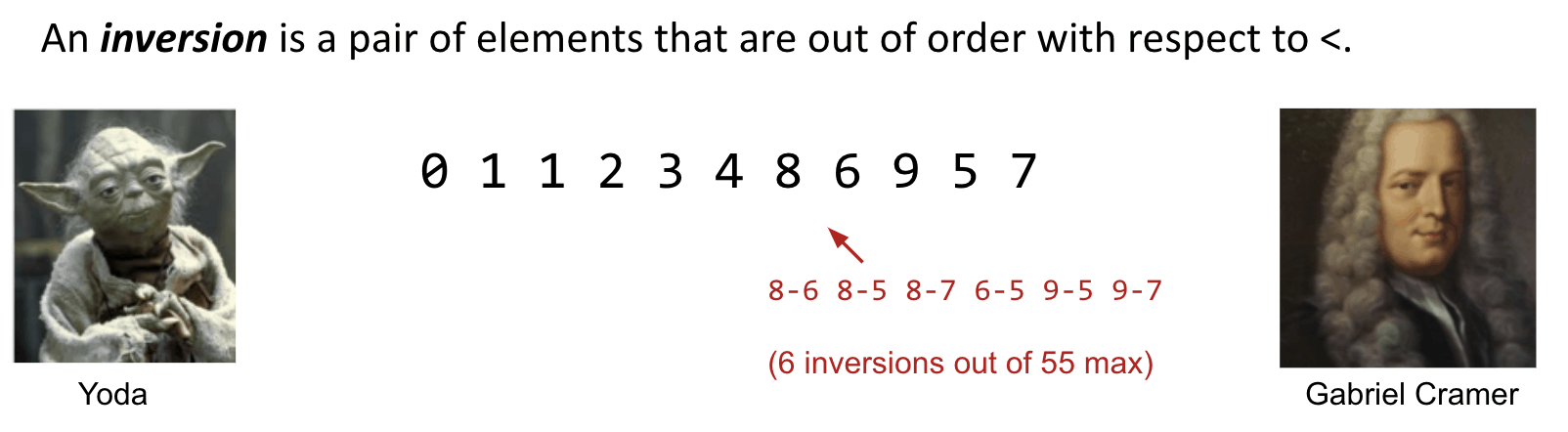
Another way to state the goal of sorting:

• Given a sequence of elements with $Z$ inversions.
• Perform a sequence of operations that reduces inversions to $0$.

Performance Definitions

Characteristics of the runtime efficiency are sometimes called the time complexity. For example, Dijkstra’s has time complexity $O(E\log{V})$.

Characteristics of the “extra” memory usage of an algorithm is sometimes called the space complexity of an algorithm. For example, Dijkstra’s ahs space complexity $\Theta(V)$ (for queue, distTo, edgeTo).

Note: A graph takes up space $\Theta(V + E)$, but we don’t count this as part of the space complexity. We don’t count input, which means it takes $\Theta(1)$ space if no additional space is used.

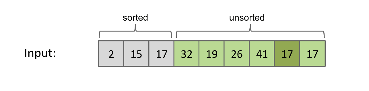
Selection Sort

Idea

Selection sorting $N$ items:

• Find the smallest item in the unsorted portion of the array.
• Move it to the end of the sorted portion of the array / the current head of the unsorted portion.
• Selection sort the remaining unsorted items.

Invariant: Everything in the far left is sorted.

Demo: link

Runtime is $\Theta(N^2)$ if we use an array.

Inefficiency: We look through entire remaining array every time to find the minimum.

Caveat

/* Selection Sort */
   sorted      unsorted
     / \    /            \
           i-------------->
Index:     0  1  2  3  4  5
Data:      3  9  8  4  6  7
           |  j----------->  update the real min
          min

Range:

• i $\in$ [0, N) (actually it could be [0, N-1))
• j $\in$ [i + 1, N)

Swap: When update finishes, swap the real min to the initial min position, i.e. i.

Handwriting: link

Code

for (int i = 0; i < N; ++i) {
  int min = i;
  for (int j = i + 1; j < N; ++j) {
    if(a[j] < a[min]) {
      min = j;
    }
  }
  swap(a, i, min);
  // swap to the first position of unsorted part
}

Heap Sort

Improvement upon selection sort.

Naive Heap Sort

Idea: Instead of re-scanning entire array looking for minimum, maintain a heap so that getting the minimum is fast.

Naive heapsorting $N$ items:

• Step 1: Insert all items into a max heap, and discard input array. Create output array. ==> $O(N\log{N})$
• Step 2: Repeat the following $N$ times.
  • Delete largest item from the max heap. ==> $O(\log{N})$
  • Put largest item at the end of the unused part of the output array. ==> $\Theta(1)$

Demo: link

Note: Memory usage is $\Theta(N)$ (worse than $\Theta(1)$ in selection sort) to build the additional copy of all of our data. However, we can eliminate this extra memory cost by In-Place Heap Sort.

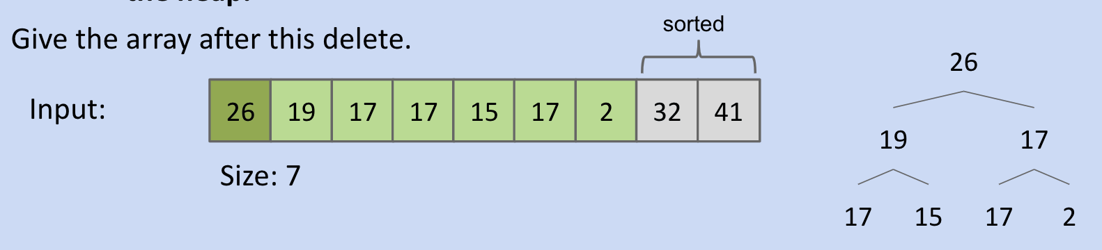
In-place Heap Sort

Wiki: An in-place algorithm is an algorithm which transforms input using no auxiliary data structure. However a small amount of extra storage space is allowed for auxiliary variables.

How do we avoid the $\Theta(N)$ space complexity?

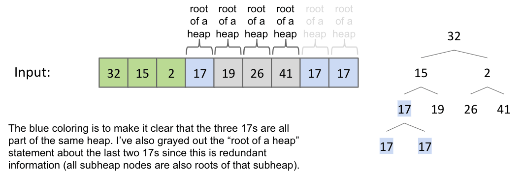
Heap sort $N$ items:

• Step 1: Bottom-up heapify input array. ==> $O(N)$
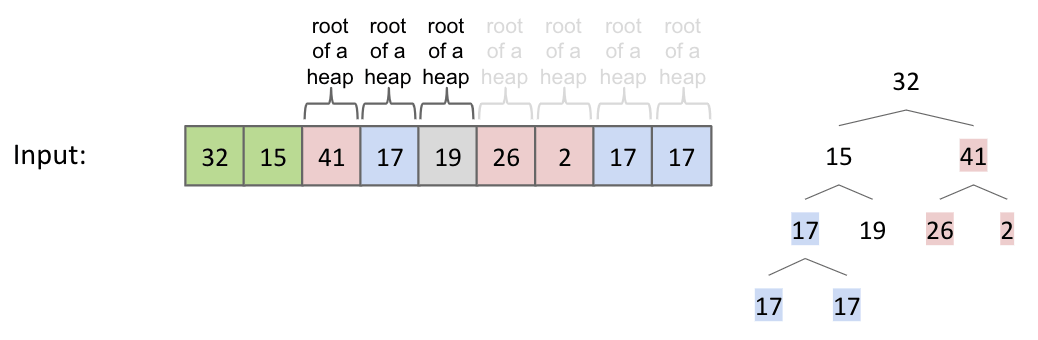
  • Sink nodes in reverse level order: sink(k)
  • After sinking, guaranteed that tree rooted at position $k$ is a heap.
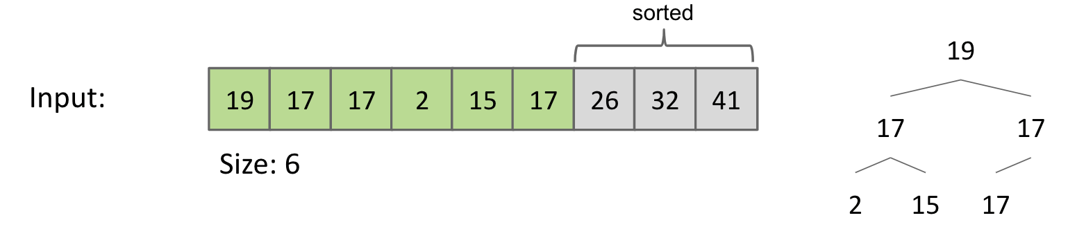
• Step 2: Delete largest item from the max heap. ==> $O(\log{N})$
  • Swapping root with the last item in the heap.
  • Sink the root if necessary.

Demo: link

Sink(2):

Punchline: Since tree rooted at position $0$ is the root of a heap, then entire array is a heap.

Note: No room to leave an unused spot since it is the original array of length $N$. We will actually use position zero for this algorithm.

Delete largest item and swap:

In-place Heapsort Complexity:

The time complexity of in-place heapsort is $O(N\log{N})$.

• Bottom-up heapification takes $N$ sink operations, each taking no more than $\log{N}$ time. Overall, the bottom-up heapification is $\Theta(N)$ in the worst case.
• Later, there are $N$ sink operations and each takes $O(\log{N})$ time.

The memory complexity is $\Theta(1)$, e.g. size variable.

Note: If we employ recursion to implement various heap operations, space complexity is $\Theta(\log{N})$ due to need to track recursive calls. But the difference between $\Theta(\log{N})$ and $\Theta(1)$ space is effectively nothing.

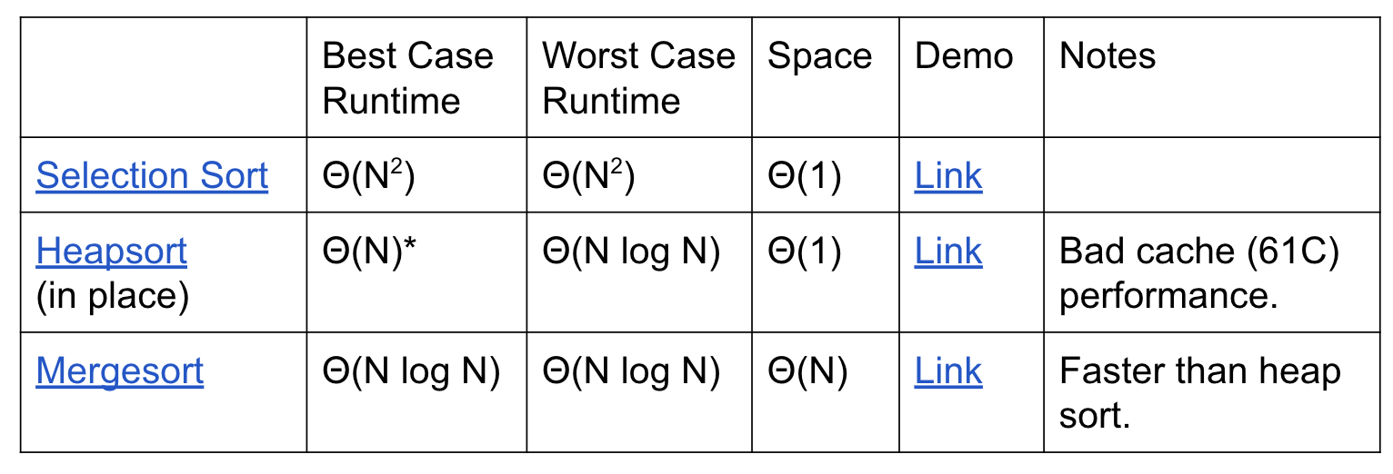
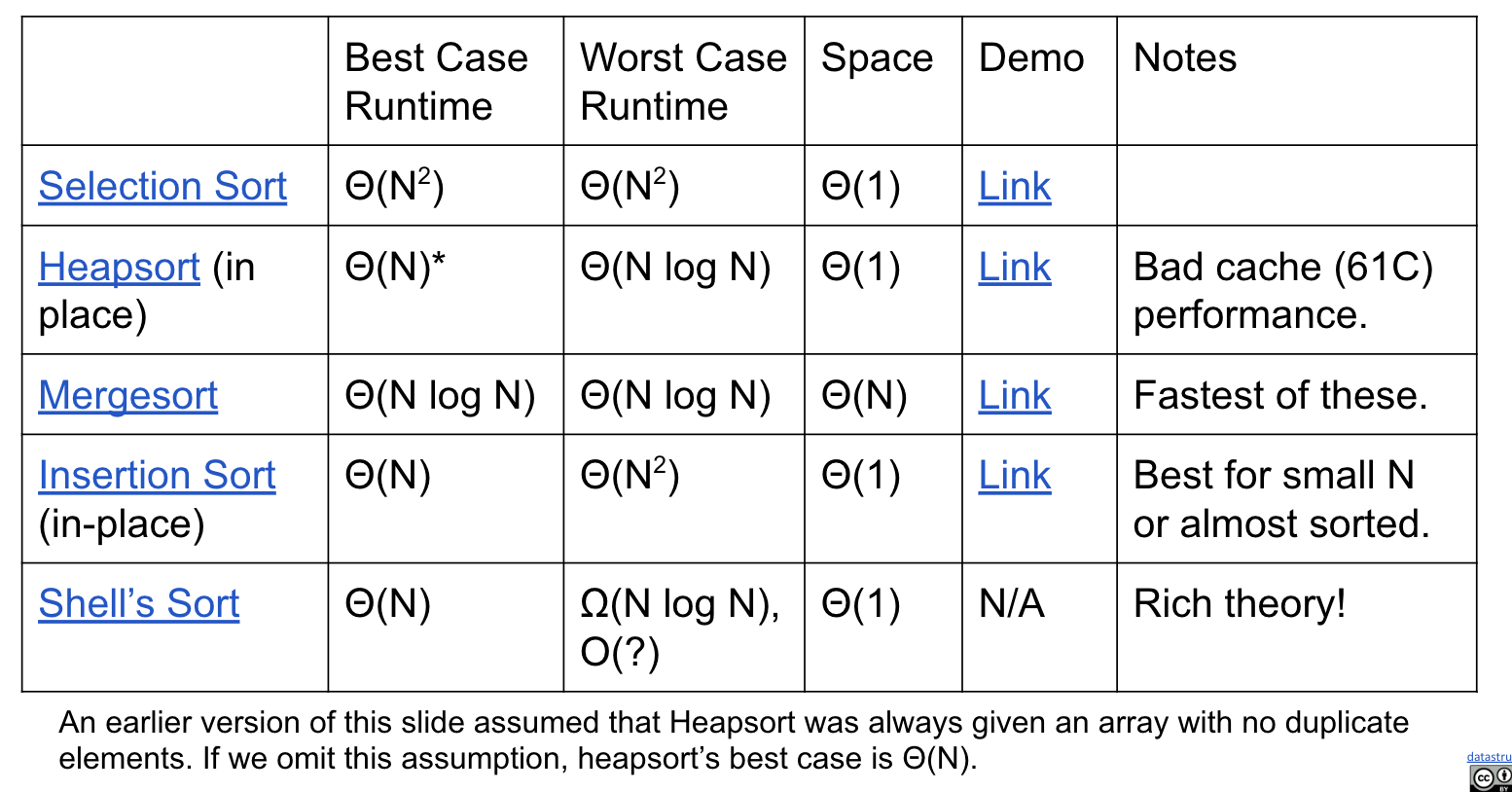
Sorts So Far (why mergesort appears early!?!??!?!??!?!?!?!?!!?!?!):

Merge Sort

Idea

Top-Down merge sorting $N$ items:

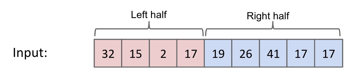
• Split items into $2$ roughly even pieces.
• Mergesort each half. (Recursive!)
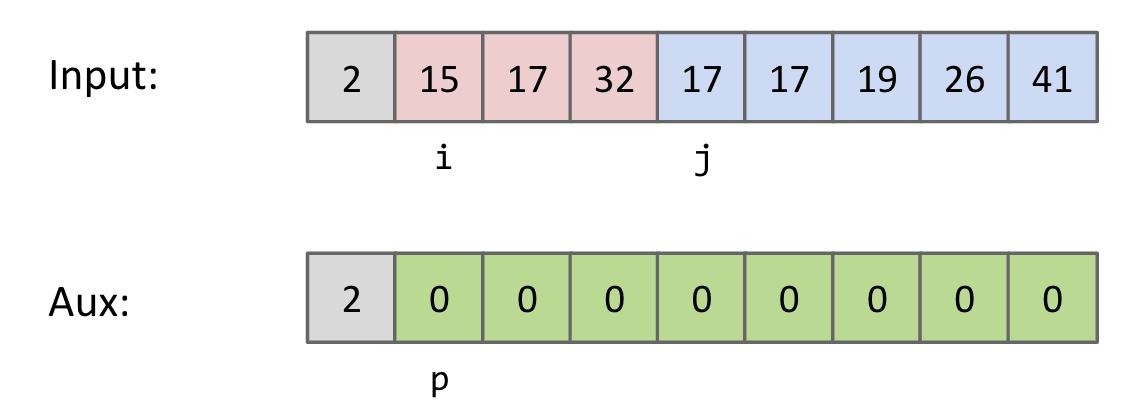
• Merge the two sorted halves to form the final result.
  • Compare input[i] < input[j].
  • Copy smaller item and increment p and i or j.

Time complexity: $\Theta(N\log{N})$
Space complexity with aux array: $\Theta(N)$

Note: Also possible to do in-place mergesort, but the algorithm is very complicated, and runtime performance suffers by a significant constant factor.

My Way (Index)

Caveat

Odd and Even Cases:

This idea can also be applied to Quicksort, Binary Search.

mid for odd and even number of items.

/* Even Case: L = 4 */
Index:  0  1  2  3
Data:   4  9  7  5
left = 0, right = 3, L = 4

mid = (left + right) / 2 = 1 => Left-Leaning
mid = (left + L) / 2 = 2 => Right-Leaning

/* Odd Case: L = 5 */
Index:  0  1  2  3  4
Data:   4  9  7  5  2
left = 0, right = 4, L = 5

mid = (left + right) / 2 = 2 => Middle
mid = (left + L) / 2 = 2 => Middle

Note: In this case, we use (left + right) / 2. So it should be Left-Leaning and we have:

• Left part: [left, mid]
• Right part: [mid + 1, right]

In merging, initializing a new array is inefficient?

Use a temp array to do merging.

Code

Three-While version:

public static void mergesort(int[] a) {
  int[] temp = new int[a.length];
  mergesort(a, temp, 0, a.length - 1);
}

private static void mergesort(int[] a, int[] temp, int left, int right) {
  if (left >= right)
    return;
  int mid = left + (right - left) / 2;
  mergesort(a, temp, left, mid);
  mergesort(a, temp, mid + 1, right);
  merge(a, temp, left, right, mid);
}

private static void merge(int[] a, int[] temp, int left, int right, int mid) {
  int i = left, j = mid + 1;
  int p = left;

  while (i <= mid && j <= right) {
    if (a[i] < a[j]) {
      temp[p++] = a[i++];
    } else {
      temp[p++] = a[j++];
    }
  }

  while (i <= mid) {
    temp[p++] = a[i++];
  }

  while (j <= right) {
    temp[p++] = a[j++];
  }

  // copy from temp[] to a[]
  for (int k = left; k <= right; k += 1) {
    a[k] = temp[k];
  }
}

For-loop version:

// Note: Be careful about the starting index
for (int k = left; k <= right; k += 1) {
  if (i > mid) { // i finished
    temp[k] = a[j++];
  } else if (j > right) { // j finished
    temp[k] = a[i++];
  } else if (a[i] < a[j]) { // subcondition
    temp[k] = a[i++];
  } else {
    temp[k] = a[j++];
  }
}

Algs4 (Creation)

Reference: algs4

Caveat

When putting elements from input to b, be careful about the offset.

Code

public static double[] mergesort(double[] input) {
  int N = input.length;
  if (N <= 1) {  // equivalent to left >= right
    return input;
  }

  double[] a = new double[N / 2];
  double[] b = new double[N - a.length]; // or N - N / 2
  for (int i = 0; i < a.length; i += 1) { // don't use N / 2
    a[i] = input[i];
  }
  for (int i = 0; i < b.length; i += 1) {
    b[i] = input[N / 2 + i]; // offset is the length of a[]
  }
  return merge(mergesort(a), mergesort(b));
}

private static double[] merge(double[] a, double[] b) {
  double[] c = new double[a.length + b.length];
  int i = 0, j = 0;
  for (int k = 0; k < c.length; k += 1) {
    if (i >=  a.length) {
      c[k] = b[j++];
    } else if (j >= b.length) {
      c[k] = a[i++];
      // The above code handle the out-of-bound cases
    } else if (a[i] <= b[j]) {
      c[k] = a[i++];
    } else {
      c[k] = b[j++];
    }
  }
  return c;
}

Insertion Sort

Two Approaches:

• Naive Approach (Move Back)
• In-Place Approach (Swapping)

Naive (Move Back)

Idea

• Starting with an empty output sequence.
• Add each item from input, inserting into output at appropriate position.

Demo: link

If output sequence contains $k$ items, worst cost to insert a single item is $k$. Might need to move everything over.

Caveat

Idea: Find the appropriate pos to insert pivot i. Move back items to provide space.

/* Insertion Sort (Naive) */
Pivot:     i----------->
Index:  0 [1] 2  3 [4] 5
Data:   3  9  5  2  1  8
        <--p (pos)
        <-----------p (pos)

Range:

• i $\in$ [1, N)
• pos $\in$ [0, i], from left to right.
  • So we have while (pos < i) { pos++; } that pos will finally stops at i.

Moving Condition:

• Know when to stop: a[pos] > a[i].
• Know when can move: !(a[pos] > a[i]).
  • Equivalent to a[pos] <= a[i].
• Combine them we have while (pos < i && !(a[pos] > a[i])).

/* Move back */
Pivot:              i-->
Index:  0 [1] 2  3 [4] 5
Data:   3  9  5  2  1  8
        <--p (pos)       // p is finalized
           <-----j

Move Back:

• Which items should be moved back: [pos, i).
  • [pos, i) => [pos, i - 1] ([i - 1] will move to [i])
  • Move back starting from right to left.
  • We have for (int j = i - 1; j >= pos; --j).

Note: Backup the item before moving back, otherwise it’ll be overwritten.

Handwriting: link

Code

public static void insertionSort(int[] a) {
  if (a == null) return;
  int N = a.length;

  for (int i = 1; i < N; i += 1) {
    int pos = 0;
    while (pos < i && !(a[i] < a[pos])) { // locate
      pos += 1;
    }
    // move back
    int beInserted = a[i];
    for (int j = i - 1; j >= pos; --j) {
      a[j + 1] = a[j];
    }
    a[pos] = beInserted;
  }
}

In-Place (Swapping)

Idea

Do everything in place using swapping.

• Designate item i $\in$ [1, N) as the traveling item.
• Swap item backwards until traveller is in the right place among all previously examined and sorted items.

Demo: link

Caveat

Idea: Swap a[j - 1] and a[j] when a[j - 1] > a[j].

/* Insertion Sort (Swapping) */
Pivot:     i----------->
Index:  0 [1] 2  3 [4] 5
Data:   3  9  5  2  1  8
        <--j
        <-----------j

Range:

• i $\in$ [1, N)
• j $\in$ (0, i], from right to left

Handwriting: link

Code

public static void sort(int[] a) {
  int N = a.length;
  for (int i = 1; i < N; i += 1) {
    for (int j = i; j > 0 && a[j - 1] > a[j]; j--) {
      swap(a, j, j - 1);
    }
  }
}

Runtime (In-Place)

Two Examples:

The purple letter is the current traveler.

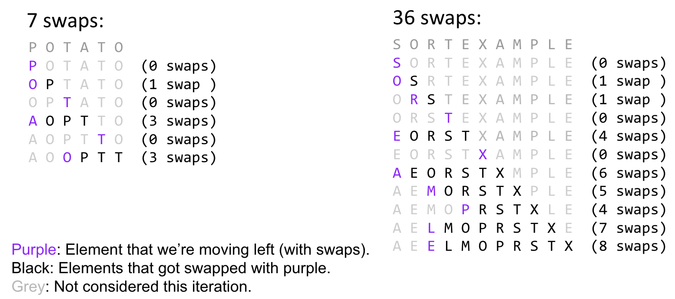
See how the travelers move forward.

Best case: $\Theta(N)$ (almost no inversion)
Worst case: $\Theta(N^2)$ (triangle)

Picking the Best Sort. Suppose we do the following:

• Read 1,000,000 integers from a file into an array of length 1,000,000.
• Mergesort these integers.
• Select one integer randomly and change it.
• Sort using algorithm $X$ of your choice.
  • Selection Sort: $O(N^2)$
  • Heap Sort: $O(N\log{N})$ (worst)
  • Merge Sort: $O(N\log{N})$ (worst)
  • Insertion Sort: $O(N^2)$ (X, this one)

Insertion Sort. Because there is only one item out of place. The times of swapping it is linear.

Heap & Merge Sorts are worst in this case since they take $O(N\log{N})$.

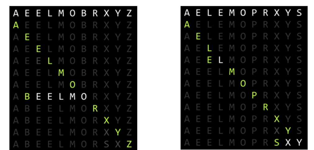
Observation: For arrays that are almost sorted, insertion sort does very little work.

• Left array: 5 inversions => 5 swaps.
• Right array: 3 inversions => 3 swaps.

Why Insertion Sort?

Sweet Spots:

On arrays with a small number of inversions, insertion sort is extremely fast.

• One exchange per inversion (and number of comparisons is similar).
• Runtime is $\Theta(N + K)$ where $K$ is number of inversions.

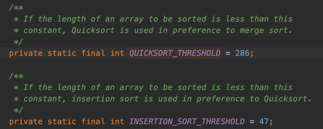
Less obvious: For small arrays ($N < 15$ or so), insertion sort is fastest.

• More of an empirical fact than a theoretical one.
• Rough Idea: Divide and conquer algorithms like heap sort / merge sort spend too much time dividing, but insertion sort goes straight to the conquest.

So, in real-world implementation of merge sort or quicksort, once the size of piece of the array is less than 15, it will switch to insertion sort. (below thresholds are different, but the idea is the same)

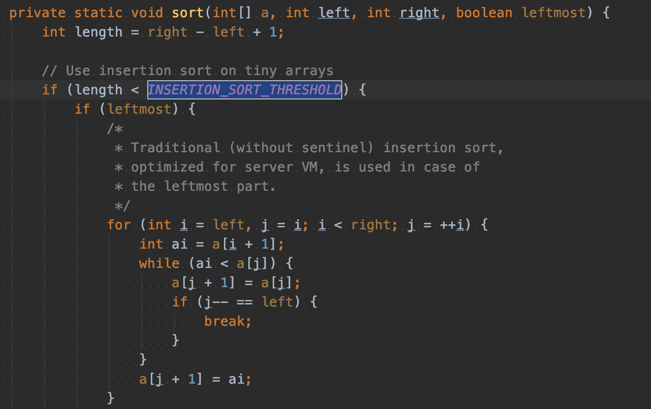
Shell’s Sort

Or Shellsort.

Idea

[algs4] Insertion sort is slow for large unordered arrays because the only exchanges it does involve adjacent entries, so items can move through the array only one place at a time.

h = 4
L  E  E  A  M  H  L  E  P  S  O  L  T  S  X  R
L-----------M-----------P-----------T
   E-----------H-----------S-----------S
      E-----------L-----------O-----------X
         A-----------E-----------L-----------R

The idea of shell sort is to rearrange the array to give it the property that taking every h-th entry (starting anywhere) yields a sorted subsequence. Such an array is said to be h-sorted. Put another way, an h-sorted array is h independent sorted subsequences. Therefore, we can move items around in the array long distances. Using such a procedure for any sequence of values of h that ends in 1 will produce a sorted array.

Big Idea: Optimize insertion sort by fixing multiple inversions at once.

• Instead of comparing adjacent items, compare items that are one stride length $h$ apart.
• Start with large stride, and decrease towards 1.
• By using large strides first, fixes most of the inversions.
• Example: $h$ = 7, 3, 1.

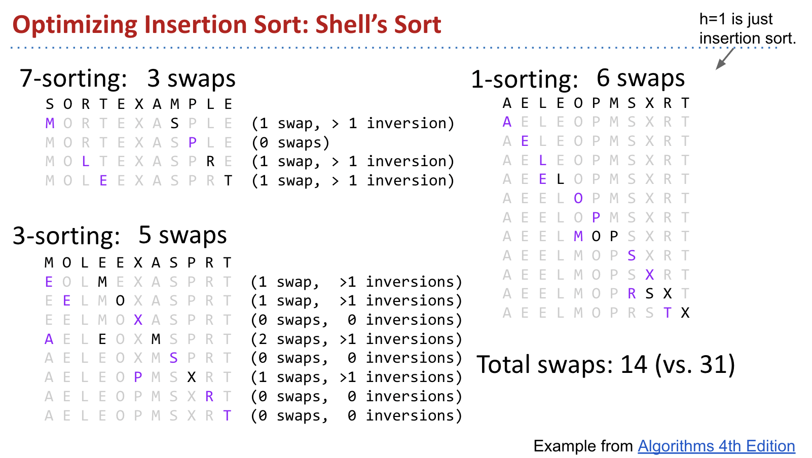
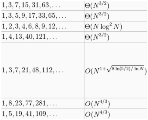
We used 7, 3, 1. Can generalize to $2^k - 1$ from some $k$ down to 1.

Worst-case Runtime: $\Theta(N^{1.5})$

Code

/*
h = 4
0  1  2  3  4  5  6  7  8  9  10 11 12 13 14 15
L  E  E  A  M  H  L  E  P  S  O  L  T  S  X  R
L-----------M-----------P-----------T
    E-----------H-----------S-----------S
      E-----------L-----------O-----------X
          A-----------E-----------L-----------R
            i                       i
j-h          j          j-h          j
            h=4
          j >= h
*/
public static void sort(int[] a) {
  int n = a.length;
  int h = 1;
  while (h < n / 3) h = 3 * h + 1;  // 1, 4, 13, 40, 121, 364, 1093, ...
  while (h >= 1) {
    // h-sort the array.
    for (int i = h; i < n; ++i) { // insert a[i] among a[i-h], a[i-2*h], a[i-3*h]
      for (int j = i; j >= h && a[j - h] > a[j]; j -= h) {
        
      }
    }
    h = h / 3;
  }
}

Sorts So Far

Ex (Guide)

Which sort do you expect to run more quickly on a reversed array, selection sort or insertion sort?

Selection Sort:

5 4 3 2 1 = N
1 4 3 2 5 = N - 1
1 2 3 4 5 = N - 2
1 2 3 4 5 = N - 3 ... 1

Insertion Sort:

5 4 3 2 1 = 1
4 5 3 2 1 = 2
3 4 5 2 1 = 3
2 3 4 5 1 = 4
1 2 3 4 5 = ... N

I think it should be Selection Sort. They both run at $O(N^2)$ (triangle), but Insertion Sort requires too many swapping.